How to use the simulated annealing toolbox of matlab
This article mainly introduces the relevant knowledge of matlab how to use the simulated annealing toolbox, the content is detailed and easy to understand, the operation is simple and fast, and has a certain reference value. I believe you will gain something after reading this article on how to use the simulated annealing toolbox in matlab. Let's take a look.
Clearclc% parameter settin
ObjectiveFunction = @ my_first_SA;% Function handle to the objective functionX0 = [0.50.5];% Starting pointlb = [- 5-5];% Lower boundub = [55];% Upper bound
Options = saoptimset ('MaxIter',500,'StallIterLim',500,'TolFun',1e-100,'AnnealingFcn',@annealingfast,'InitialTemperature',100,'TemperatureFcn',@temperatureexp,'ReannealInterval',500,'PlotFcns', {@ saplotbestx, @ saplotbestf, @ saplotx, @ saplotf,@saplottemperature});% start running simulated annealing to solve [XMae Fval] = simulannealbnd (ObjectiveFunction,X0,lb,ub,options); function y = my_first_SA (x)
% this is the objective function
% Rastrigin's functiony = 20 + x (1) ^ 2 + x (2) ^ 2-10 * (cos (2*pi*x (1)) + cos (2*pi*x (2); this is the end of the article on "how to use the matlab simulated annealing toolbox". Thank you for reading! I believe you all have a certain understanding of the knowledge of "how to use the matlab simulated annealing toolbox". If you want to learn more, you are welcome to follow the industry information channel.